Laminar flat-channel flow
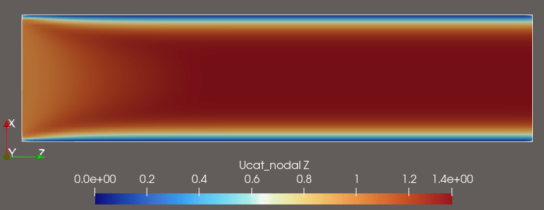
Flow at Re = 200 moves through a straight rectangular channel with no-slip walls, a constant-velocity inlet, and a conservative outlet.
- 9 × 9 × 17
- grid cells
- 20
- timesteps
- 2
- MPI ranks
|
PICurv 0.1.0
A Parallel Particle-In-Cell Solver for Curvilinear LES
|

|
Create, validate, run, and inspect a complete
PICurv case from a clean workspace. Cropped preview · Ucat_nodal at step 20 Flow at Re = 200 moves through a straight rectangular channel with no-slip walls, a constant-velocity inlet, and a conservative outlet. Dual-time Picard–Jameson RK advances momentum. FGMRES with a three-level geometric-multigrid preconditioner solves the pressure correction.
 Quick Start
Your first simulation.
Laminar flat-channel flow
Dual-time + multigrid
One case. Four clear moves.
PICurv must be built with an MPI runtime available. Load the project environment:
If picurv --help fails, complete the Installation guide. Run the remaining commands from the workspace where the new case should live.
Initialize the checked-in flat-channel template and enter the new case directory:
A successful initialization ends with:
[SUCCESS] Case directory is ready.
          Runtime binaries (simulator, postprocessor) are resolved from bin/ automatically.
This run uses four profiles:
quickstart_flat_channel.yml
Grid and physics.
Imp-MG-Standard.yml
Numerical methods.
quickstart_Standard_Output.yml
Logs and checkpoints.
quickstart_standard_analysis.yml
VTK output.
Check the four profiles together:
The final line is:
[SUCCESS] Validation completed for 5 file(s).Launch the 20-step case on two MPI ranks and post-process its final checkpoint:
The quickstart grid contains 9 x 9 x 17 cells. A completed run ends with:
[INFO] Created new self-contained run directory:
       runs/quickstart_flat_channel_<timestamp>

Progress: [==================================================] 100% (Step 20/20)
[SUCCESS] Execution finished successfully.

RUN SUMMARY
  Stages          : solve, post-process
  Solver MPI procs: 2
  Post MPI procs  : 2
  Steps run       : 20
Post output : <run.visualization>/<recipe_id>/The postprocessor writes one VTK structured-grid file for the final step, and the conductor writes a collection containing its checkpoint physical time:
Open eulerian_data.pvd in ParaView, add a Slice, and color it by Ucat_nodal:
Use the Visualization tutorial for the complete ParaView workflow and other output fields.
This Quick Start is deliberately small, but it does not use a special execution path. Every PICurv simulation follows the same workflow: define its case and supporting profiles, validate them together, materialize a self-contained run, execute the MPI solver, and post-process checkpoints into analysis-ready output.
The grid, physics, solver, monitoring, and analysis choices can change from one case to another; this simulation workflow stays the same.
For a failed command or incomplete run, use Troubleshooting.
 1.9.8
1.9.8